Confusion Matrices

A confusion matrix is a tabular summary of how well a classification model's predictions match the actual labels. It compares the predicted classes with the true classes, allowing you to visualize the performance of your algorithm.

In the realm of data science and machine learning, evaluating the performance of classification models is crucial. One fundamental tool for this purpose is the confusion matrix. Despite its seemingly perplexing name, the confusion matrix provides a clear snapshot of your model's performance, helping you understand where it excels and where it falters.

In this article, we'll demystify confusion matrices, explore their components, and demonstrate how they can be used to assess classification models effectively.

Structure of a Confusion Matrix

For a binary classification problem (i.e., classifying data into two classes), a confusion matrix is a 2x2 table that looks like this:

• True Positive (TP): Correctly predicted positives.

• True Negative (TN): Correctly predicted negatives.

• False Positive (FP): Incorrectly predicted positives (Type I error).

• False Negative (FN): Incorrectly predicted negatives (Type II error).

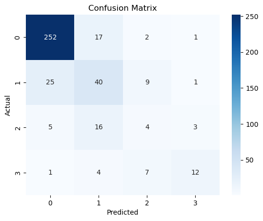
Confusion Matrices have as many "classes" as there are categories in the predictive model. Below is an example 4-class confusion matrix showing predicted versus actual quartiles of violent crime distribution across 1,994 cities in the United States, with 0 being lowest (0-25%), 1 low (26-50%), 2 elevated (51-75%), and 3 highest (76-100%). 

For those who have not seen a confusion matrix before, let me orient you. Over on the left (y-axis) are the actual violent crime quartiles of the cities in the test data segment, and on the bottom are the model-predicted quartiles. So, the top left box shows the count of test records (cities) for which both the predicted (x-axis) and actual (y-axis) violent crime quartile was 0-25%. On the top-right, the "1" means that my model predicted a city in the test data to be in the highest quartile of violent crime (76-100%) but it was actually in the lowest (0-25%).

Confusion matrices allow for much more nuanced analyses of data models than overall accuracy statistics.

Of note, the total number in the matrix is only 399. This is because it represents the test partition of provided data, 20% of the total records present in the analyzed dataset. The machine learning model trained on a random 80% of the base data, and the optimized model was then applied to the remainder to test how well the model performed on data it had not seen.

Confusion matrices are important to understand how data models compare to the actual world. While accuracy (the proportion of correct predictions) is a common metric, it can be misleading on its own, especially with imbalanced datasets where one class significantly outnumbers the others.

For example, imagine a disease afflicting 1 in every 100 people. Since 99% of the population is not affected by the disease, a data model that predicts no disease for everyone would still be 100% accurate.     

Confusion matrices provide more detail, showing the breakdown of correct and incorrect predictions for each class. Several metrics based on confusion matrix data clarify model performance. Remember: TP means true positive and TN means true negative.

1. Accuracy

The overall correctness of the model.

2. Precision

The proportion of positive identifications that were actually correct.

3. Recall (Sensitivity or True Positive Rate)

The proportion of actual positives that were correctly identified.

4. Specificity (True Negative Rate)

The proportion of actual negatives that were correctly identified.

5. F1 Score

The harmonic mean of precision and recall.

A Simple Example to Illustrate

Suppose you're building a model to detect fraudulent transactions. Out of 1,000 transactions:

• 950 are legitimate (Negative class).
• 50 are fraudulent (Positive class).

Your model predicts:

• 920 legitimate transactions correctly (TN).
• 30 legitimate transactions incorrectly as fraudulent (FP).
• 40 fraudulent transactions correctly (TP).
• 10 fraudulent transactions incorrectly as legitimate (FN).

Confusion Matrix for This Scenario:

Calculated Metrics:

• Accuracy: (40 + 920) / 1,000 = 96%
• Precision: 40 / (40 + 30) ≈ 57.14%
• Recall: 40 / (40 + 10) = 80%
• F1 Score: 2 * (0.5714 * 0.8) / (0.5714 + 0.8) ≈ 66.67%

Interpretation:

• High Accuracy: The model seems accurate, but this is largely due to the high number of legitimate transactions.
• Precision: Only about 57% of the transactions flagged as fraudulent are actually fraudulent.
• Recall: The model catches 80% of fraudulent transactions.
• F1 Score: Provides a balance between precision and recall.

As you can see, confusion matrices are a critical way to evaluate the performance of classification models in data science and machine learning. By providing a clear snapshot of correct and incorrect predictions for each class, confusion matrices enable data scientists to identify areas where their model excels and falters.

The various metrics derived from confusion matrix data, such as accuracy, precision, recall, specificity, and F1 score, offer a more nuanced understanding of model performance than overall accuracy statistics alone. These metrics provide valuable insights into the strengths and weaknesses of a classification model, helping data scientists refine their models to improve their predictive power.