Global & Local Optima

Optimization is a critical component of data science, mathematics, and decision-making fields where achieving the best possible outcome given constraints is essential. Key to this process is distinguishing between global and local optima. This article delves into these concepts, offering illustrative Python code examples with calculus principles to visualize these optima and apply optimization routines practically.

What Are Global and Local Optima?

Global Optimum: The pinnacle of optimization, a global optimum is the best possible solution over the entire domain of a function, representing either the absolute minimum or maximum value. For a function ( f(x) ) over a domain ( D ), a point ( x^* ) is the global minimum if:

Local Optimum: A local optimum is the highest or lowest point in a specific, localized region of the domain. While optimal within this neighborhood, it may not be the best among all possible solutions. Formally, ( x^\dagger ) is a local minimum if there exists a neighborhood ( N ) such that:

Challenges in Finding Global Optima

Finding global optima is challenging due to the presence of multiple local optima. Optimization algorithms, especially those like gradient descent, risk getting 'trapped' in local optima, mistaking them for the global one. This is particularly problematic in high-dimensional, non-convex landscapes where understanding the global shape is complicated.

Calculating Optima Using Calculus

Calculus provides a powerful toolset to identify local optima through evaluating critical points and applying derivative tests. Below is a Python example illustrating these methods.

import numpy as np
import matplotlib.pyplot as plt

# Define the function
def f(x):
    return x**4 - 3*x**3 + 2

# First derivative
def df(x):
    return 4*x**3 - 9*x**2

# Second derivative
def d2f(x):
    return 12*x**2 - 18*x

# Use derivative tests to find critical points
critical_points = np.roots([4, -9, 0])

# Evaluate critical points to find minima and maxima
for point in critical_points:
    second_derivative = d2f(point)
    if second_derivative > 0:
        print(f"Local minimum at x = {point}")
    elif second_derivative < 0:
        print(f"Local maximum at x = {point}")

# Plot the function
x = np.linspace(-1, 3, 400)
y = f(x)
plt.plot(x, y, label="f(x)")
plt.scatter(critical_points, f(critical_points), color='red')  
plt.title("Global and Local Optima")
plt.xlabel("x")
plt.ylabel("f(x)")
plt.legend()
plt.show()

Explanation of the Code

• Function Definition: The function ( f(x) = x^4 - 3x^3 + 2 ) is analyzed.

• Derivative Calculations:

• ( f'(x) = 4x^3 - 9x^2 ), the first derivative, is employed to find where the slope is zero, pinpointing critical points.

• ( f''(x) = 12x^2 - 18x ), the second derivative, is used to classify critical points as minima or maxima.

• Critical Points: Solved by setting the first derivative to zero.

• Second Derivative Test: Determines the nature of each critical point based on the second derivative's sign.

• Visualization: The function graphically plots critical points to illustrate local minima and maxima.

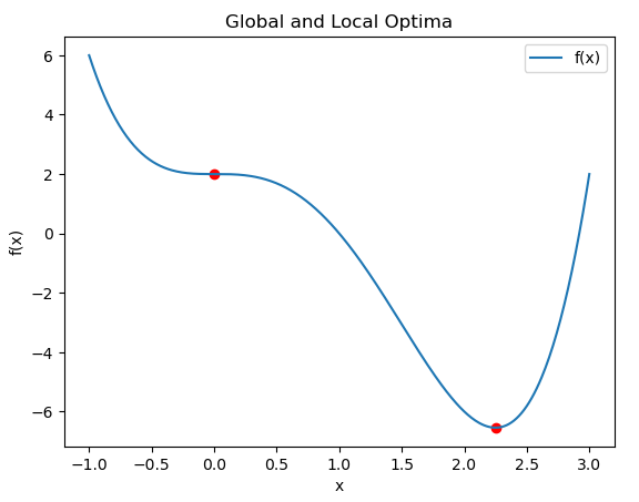
For those unfamiliar with Calculus, focus on the above graph if f(x). The blue line represents the function f(x), with changes in its slope reflecting both rising and falling trends as the value of x changes. You'll notice that a local maximum is around 0, at which a red dot marks a peak in the graph. (This flattening out is actually a "saddle point.") Since the graph, extending down to -1, shows f(x) the blue line moving even higher, this is a local maximum rather than a global one. Similarly, the lowest point across the entire graph occurs when x is near 2.2, but that red dot marks the global minimum of f(x) within the given range.

More complex instantiations of this approach are used to optimize multiple simultaneous bounding functions, making the output extremely practical. For example, in machine learning, this technique can be applied to tune hyperparameters across multiple models simultaneously, balancing accuracy, computational cost, and memory usage. In engineering, multi-objective optimization might be used to design materials that are both strong and lightweight, with each objective function representing a different desired property. Similarly, in finance, portfolio optimization can use multiple bounding functions to balance risk, return, and liquidity, providing investors with an efficient frontier of optimal choices.

Optimization is the process of finding the best solution to a problem within a set of constraints. It involves selecting values for variables to maximize or minimize a particular outcome, like minimizing costs or maximizing efficiency. In essence, optimization helps us make the most effective use of resources to achieve a desired goal.

In practice, multi-objective optimization is a powerful means of balancing competing objectives, maximizing efficiencies, and minimizing losses. By leveraging this technique across various fields, data science has uncovered innovative solutions that meet complex requirements and maximize effective use of resources. Ultimately, the application of multi-objective optimization has far-reaching implications for problem-solving, contributing to significant progress in areas where efficiency, practicality, and innovation converge.