Decision Tree Classifiers

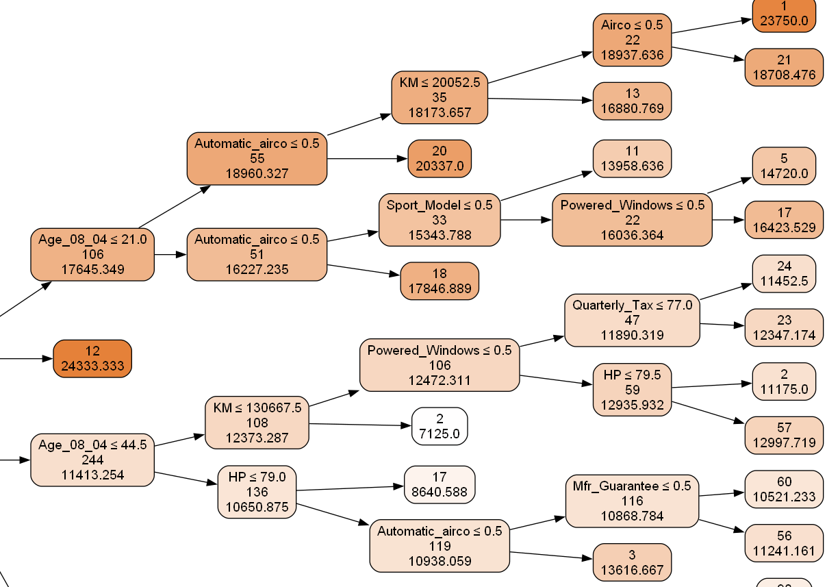
Decision tree classifiers are popular in machine learning for both classification and regression tasks. They use a rule-based, hierarchical structure that makes their decision-making process straightforward and interpretable, which contributes to their widespread use in practical applications.

A decision tree classifier is a model that makes predictions based on a series of decision rules derived from the data's features.

• Structure: It consists of nodes representing decisions, starting from a root node branching out into leaves, which indicate the ultimate prediction or classification outcome.

• Splitting Criteria: The decision-making process at each node uses metrics like Gini impurity, information gain, or variance reduction to determine the optimal feature split.

• Overfitting Solutions: While effective, decision tree models can overfit on training data, capturing more noise than abstracted signal from the data. Techniques like pruning, controlling tree depth, or employing ensemble methods like Random Forests are utilized to combat this issue.

Example Python Code

Categorical Data: Classification Task

In this example, we load the Iris dataset, split it into training and testing sets, and then train a random forest classifier. The model's performance is evaluated using a classification report and accuracy score. 

from sklearn.datasets import load_iris

from sklearn.tree import DecisionTreeClassifier

from sklearn.model_selection import train_test_split

from sklearn.metrics import accuracy_score

# Load the dataset

data = load_iris()

X_train, X_test, y_train, y_test = train_test_split(

    data.data, data.target, test_size=0.3, random_state=42

)

# Train the classifier

clf = DecisionTreeClassifier()

clf.fit(X_train, y_train)

# Evaluate the performance

y_pred = clf.predict(X_test)

accuracy = accuracy_score(y_test, y_pred)

print(f"Accuracy: {accuracy:.2f}")

Continuous Data: Regression Task

In this example, we use the Boston Housing dataset is a classic dataset in machine learning and statistics, often used to demonstrate regression techniques. It contains information collected by the U.S. Census Service concerning housing in the area of Boston, Massachusetts. This dataset is primarily used to predict housing prices based on various features of the neighborhood.

from sklearn.datasets import load_boston

from sklearn.tree import DecisionTreeRegressor

from sklearn.model_selection import train_test_split

from sklearn.metrics import mean_squared_error

# Load the dataset

boston = load_boston()

X_train, X_test, y_train, y_test = train_test_split(

    boston.data, boston.target, test_size=0.3, random_state=42

)

# Train the regressor

reg = DecisionTreeRegressor()

reg.fit(X_train, y_train)

# Evaluate the performance

y_pred = reg.predict(X_test)

mse = mean_squared_error(y_test, y_pred)

print(f"Mean Squared Error: {mse:.2f}")

The Boston dataset was removed in the latest version of sklearn, but the same below Python code will work if you replace the two instances of 'load_boston' with 'fetch_california_housing' (and, if you want, the name of the dataset variable from 'boston' to something else, like 'california' for example.

from sklearn.datasets import fetch_california_housing

from sklearn.tree import DecisionTreeRegressor

from sklearn.model_selection import train_test_split

from sklearn.metrics import mean_squared_error

# Load the dataset

california = fetch_california_housing()

X_train, X_test, y_train, y_test = train_test_split(

    california.data, california.target, test_size=0.3, random_state=42

)

# Train the regressor

reg = DecisionTreeRegressor()

reg.fit(X_train, y_train)

# Evaluate the performance

y_pred = reg.predict(X_test)

mse = mean_squared_error(y_test, y_pred)

print(f"Mean Squared Error: {mse:.2f}")

Example R Code

Categorical Data: Classification Task

# Load required libraries

library(datasets)

library(caret)

library(rpart)

# Load the dataset

data(iris)

set.seed(42)

# Split the data into training and test sets

trainIndex <- createDataPartition(iris$Species, p = 0.7, list = FALSE)

trainData <- iris[trainIndex, ]

testData <- iris[-trainIndex, ]

# Train the classifier

clf <- rpart(Species ~ ., data = trainData, method = "class")

# Predict on the test data

y_pred <- predict(clf, testData, type = "class")

# Evaluate the performance

accuracy <- sum(y_pred == testData$Species) / nrow(testData)

print(sprintf("Accuracy: %.2f", accuracy))

After loading the data, the createDataPartition function from the caret package splits the data, after which rpart is used to create a decision tree model similar to Python's DecisionTreeClassifier. Finally, we make predictions on the test data, comparing predicted values to actuals in testData$Species. 

Continuous Data: Regression Task

The Boston dataset is available in the MASS package for R, so we use it load the data. After partitioning the data with caret, we train the model with method = "anova" for regression. Evaluation of predictions made on the test data utilize Mean Squared Error (MSE), calculated manually by squaring the differences, summing, and averaging.

Decision tree classifiers are imminently useful. If you're interested in learning more, check out the data projects on this site and these additional online resources:

• https://www.geeksforgeeks.org/building-and-implementing-decision-tree-classifiers-with-scikit-learn-a-comprehensive-guide/ 

• https://towardsdatascience.com/decision-tree-classifier-explained-in-real-life-picking-a-vacation-destination-6226b2b60575 

• https://www.datacamp.com/tutorial/decision-tree-classification-python